Aim
The aim of this project was to attain a thorough overview of jobs relating to business intelligence analysis. I wanted to identify the number of jobs, typical salaries and key competencies required for a range of similar roles using a variety of techniques.
Selenium is a powerful tool to extract data from websites. I wrote a code in Python to use Selenium to extract relevant details about job listings on Indeed.
View web scraping code:
driver = webdriver.Chrome()
processed_job_ids = []
data = []
previous_date = None  # Variable to store the previous date

def calculate_posted_date(date_str):
    if "Just posted" in date_str or "Today" in date_str:
        return datetime.datetime.now().strftime('%Y-%m-%d')
    elif "day" in date_str:
        days_ago = int(re.search(r'\d+', date_str).group())
        return (datetime.datetime.now() - datetime.timedelta(days=days_ago)).strftime('%Y-%m-%d')
    elif "days ago" in date_str:
        days_ago = int(re.search(r'\d+', date_str).group())
        return (datetime.datetime.now() - datetime.timedelta(days=days_ago)).strftime('%Y-%m-%d')
    else:
        return '1900-01-01'

for country in ['uk', 'ch']:
    for i in range(0, 500, 10):
        if country == 'uk':
            url = f'https://uk.indeed.com/jobs?q=Business+intelligence&l=England&sort=date&start={i}'
        elif country == 'ch':
            url = f'https://ch.indeed.com/Stellen?q=business+intelligence&sort=date&lang=en&vjk=f30739b891280aba&start={i}'
        driver = webdriver.Chrome()
        driver.get(url)

        job_listings = driver.find_elements(By.CLASS_NAME, 'job_seen_beacon')

        for job in job_listings:
            Job_ID = job.find_element(By.XPATH, './/a').get_attribute('data-jk')

            # Check if the Job ID has already been processed
            if Job_ID in processed_job_ids:
                continue

            Title = job.find_element(By.XPATH, './/span[starts-with(@title, "")]').text
            Location = job.find_element(By.CLASS_NAME, "companyLocation").text
            Company = job.find_element(By.CLASS_NAME, "companyName").text

            # Wait for the "date" element to be visible
            date_element = WebDriverWait(driver, 10).until(EC.visibility_of_element_located((By.CLASS_NAME, "date")))

            # Get the text of the "date" element
            Date_str = date_element.text

            Date_str = job.find_element(By.CLASS_NAME, "date").text
            Date = calculate_posted_date(Date_str)

            Country = country
            try:
                Link = job.find_element(By.XPATH, './/a[starts-with(@id, "job_") and contains(@class, "jcs-JobTitle")]').get_attribute('href')
            except:
                Link = ""
            try:
                Salary = job.find_element(By.CLASS_NAME, "attribute_snippet").text
            except:
                Salary = ""

            if Date != previous_date:
                print("New date:", Date)
                previous_date = Date

            driver.execute_script("window.open('');")
            driver.switch_to.window(driver.window_handles[1])
            if Link:
                driver.get(Link)
            try:
                job_description = driver.find_element(By.ID, "jobDescriptionText").text
            except:
                job_description = ""

            # Append the job data to the list only if it's not a duplicate
            if Job_ID not in processed_job_ids:
                data.append([Country, Job_ID, Title, Location, Company, Date_str, Date, Link, Salary, job_description])
                processed_job_ids.append(Job_ID)

            driver.close()
            driver.switch_to.window(driver.window_handles[0])

        driver.quit()

df = pd.DataFrame(data=data, columns=['Country', 'Job ID', 'Title', 'Location', 'Company', 'Date_str', 'Date', 'Link', 'Salary', 'Description'])
My code extracted a total of 2149 relevant jobs with 1554 unique titles across 748 locations.
Job ID         2149
Title          1553
Location        748
Company        1154
Date             62
Link           2137
Salary          416
Date_str         87
Description    2105
Country           2
dtype: int64
To investigate the key skills/software knowledge required for these jobs I extracted the descriptions of these jobs and searched through them for specific keywords. Here are the results:

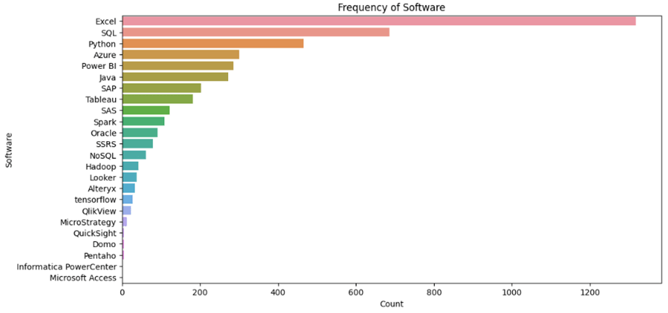
“Reporting” is more commonly mentioned by some considerable distance, followed by “AI/ML” and “dashboarding”. In terms of software, Excel takes the lead, followed by SQL, Python, Azure and Power BI.
Next I wanted to explore whether or not there are any associations to be found between these specific keywords and the respective job titles. The problem here is that there were 1554 unique job titles, so I needed to refine these into a more manageable number of ‘job categories’. To find out what these categories should be, I looked for patterns in the job titles. First I identified the most common words extracted earlier:
View job categorization code:
# Create a new column with individual words from the job title
df_titlewords=df['Title'].str.split()
# Explode the 'Title_Words' column to separate each word into a separate row
df_words = df_titlewords.explode('Title')
import pandas as pd
df_words = df_words.to_frame(name='Words')words_to_remove = ['-', '/', '–', '—', '−', '−', 'in', '(m/f/d)', 'and', 'of', 'with', '&', '', 'Position', '(PhD.', 'Candidate)']
df_words = df_words[~df_words['Words'].isin(words_to_remove)]
upper_quartile = df_words['Words'].value_counts().quantile(0.98)
# Filter the dataframe to include words within the upper quartile
words_in_upper_quartile = df_words['Words'].value_counts()[df_words['Words'].value_counts() >= upper_quartile].index.tolist()
df_upper_quartile = df_words[df_words['Words'].isin(words_in_upper_quartile)]
# Get the word frequencies
word_frequencies = df_upper_quartile['Words'].value_counts()
# Sort the words and frequencies in descending order
sorted_words = word_frequencies.index.tolist()
sorted_frequencies = word_frequencies.tolist()
# Set up the figure and axis
fig, ax = plt.subplots(figsize=(10, 8))
# Generate the stacked bar chart
ax.bar(sorted_words, sorted_frequencies)
ax.set_title('Frequency of Title Words (Upper Quartile)')
ax.set_xlabel('Title Words')
ax.set_ylabel('Count')
ax.tick_params(axis='x', rotation=90)
plt.show()

Then I used a co-occurrence matrix to rank the most common pairs of words:
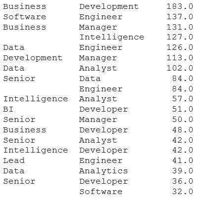
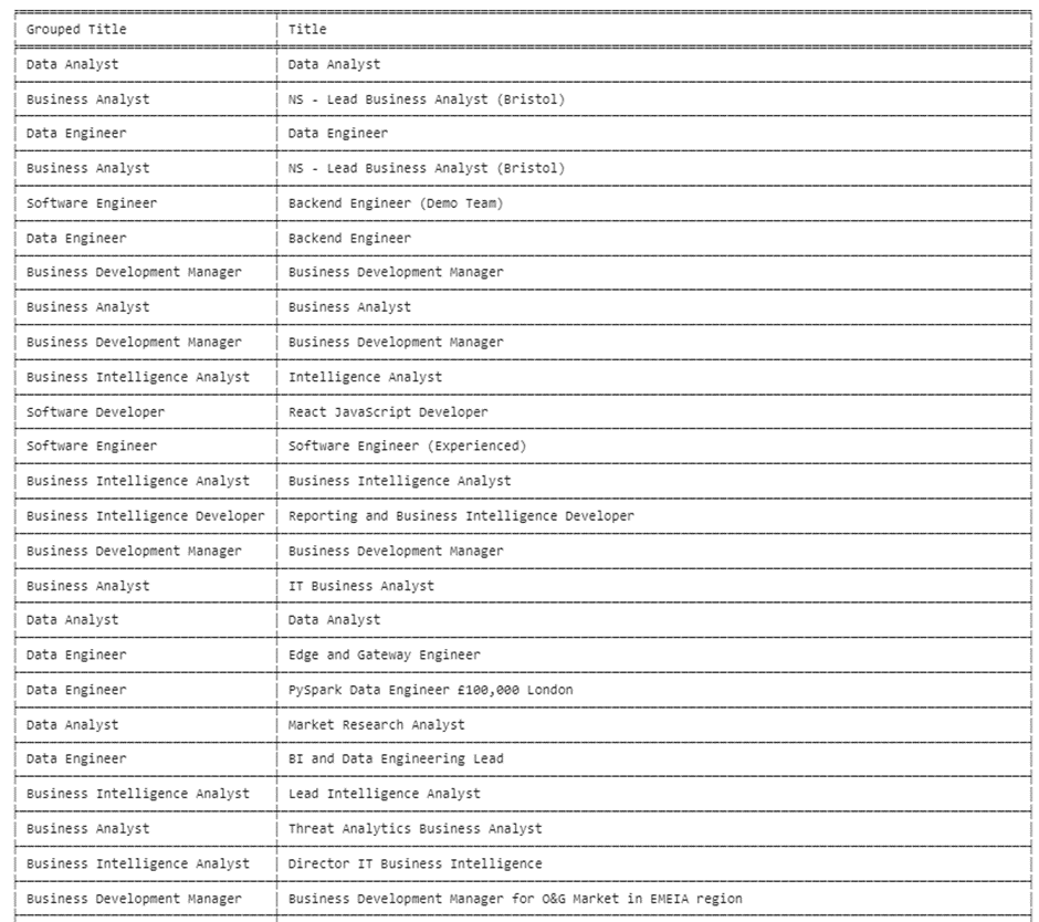
Using this information I generated 16 job titles and used a package in python to sort the 1553 unique job titles into each of these (and other for those which did not meet the similarity threshold). The process was not perfect, but it was good (and saved me trawling through 1553 job titles!). Here is a snippet of the output:
and here are the resulting numbers for each of the 16 types of job:

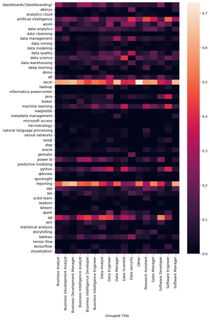
Then I used a heatmap to visualize the common associations between the keywords found in the job descriptions and these 16 job titles. I was particularly interested in any unique features on the vertical axis which would set one category apart from another.

We can already see some interesting differences, for example, “Data security” seems to require a very different skillset to the other job categories, and it looks like Data engineers require the broadest skillset. To enhance these differences I used, a TF-IDF approach. TF-IDF stands for Term Frequency-Inverse Document Frequency. It is a numerical statistic used in information retrieval and text mining to evaluate the importance of a term within a document. In this case, this approach measures the frequency of a keyword in association with a specific job category, and the rarity of that word over all of the job categories and assigns it a corresponding score. This score is then used to produce another heatmap which will really highlight the more unique features of each job category. Here is the result:
View web scraping code:
from sklearn.feature_extraction.text import TfidfVectorizer
# Define a custom tokenizer function that splits the text on whitespace only
def custom_tokenizer(text):
    return text.split(":")
# Group the data by "Grouped Title" and join the "Combined" words into a single string for each group
grouped = df_combined.groupby('Grouped Title')['Combined'].apply(':'.join).reset_index()
# Create a TF-IDF vectorizer with the custom tokenizer and fit it on the grouped data
vectorizer = TfidfVectorizer(tokenizer=custom_tokenizer)
tfidf_matrix = vectorizer.fit_transform(grouped['Combined'])
# Create a DataFrame with the TF-IDF scores for each word and "Grouped Title"
tfidf_df = pd.DataFrame(tfidf_matrix.toarray(), index=grouped['Grouped Title'], columns=vectorizer.get_feature_names_out())
# To visualize the result, you can use a heatmap
import seaborn as sns
fig, ax = plt.subplots(figsize=(8, 13))
sns.heatmap(tfidf_df.T, ax=ax)
Towards the end of this project I looked at the salary information (where available). I plotted the count of the jobs available and overlaid it with boxplots showing the median salary (and the 50th percentile in red) for each job category. The result gives a nice summary of two key features of demand – salary and number of job postings.
View job count/salary visualization code:
import seaborn as sns
import matplotlib.pyplot as plt
# Filter the dataframe to include only UK jobs
uk_df_clean = df_clean[df_clean['Country'] == 'uk']
# Calculate the median salary for each job category
median_salary = uk_df_clean.groupby('Grouped Title')['mid_salary'].median().sort_values(ascending=False)
# Remove specific job categories from the median_salary series
exclude_categories = ['Sales Manager', 'Software Manager']
median_salary = median_salary.drop(exclude_categories)
# Reverse the order of the medians
median_salary = median_salary[::-1]
# Filter the dataframe to exclude the specified job categories
filtered_df = uk_df_clean[~uk_df_clean['Grouped Title'].isin(exclude_categories)]
# Create the boxplot using Seaborn with ordered and filtered job categories
plt.figure(figsize=(10, 8))
sns.boxplot(data=filtered_df, x='Grouped Title', y='mid_salary', order=median_salary.index)
plt.xticks(rotation=90)
plt.xlabel('Job Category')
plt.ylabel('Salary')
plt.title('Salary Distribution by Job Category (Ordered by Median Salary, UK Jobs)')
plt.show()
plt.figure(figsize=(10, 8))
sns.countplot(data=filtered_df, x='Grouped Title', order=median_salary.index)
plt.xticks(rotation=90)
plt.xlabel('Job Category')
plt.ylabel('Count')
plt.title('Count of Jobs by Job Category (UK Jobs)')
plt.show()

Finally, I exported the data to Power BI to present additional visuals. Firstly, I took a quick look at the opportunities for remote or on-site work, which revealed that the majority of jobs require on-site work. Notably, there are approximately three times more jobs offering hybrid work compared to remote work.

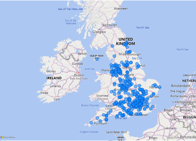
As you would expect the jobs are focused around the cities in England. We can see some clustering around the top 3 largest cities in the England; London, Birmingham and Manchester.
For comparison, I did the same for jobs in Switzerland. As expected, most of the jobs can be found around the major cities in the North of Switzerland, particularly Zürich, Basel Geneva.


Conclusion
This was a fun project to work on and a learned a couple of new techniques. It was interesting to explore the distinctions between the jobs types based on the keywords found in the job descriptions. So far this project represents about 3 months worth of data, but I will continue to add to it.
Later I would like to explore how the demand for these different jobs changes over time. I am expecting more requirements in the direction of machine learning and AI, as well as cloud based technologies as these relatively new (or at least much more publicly accessible) technologies become more widely adopted.
