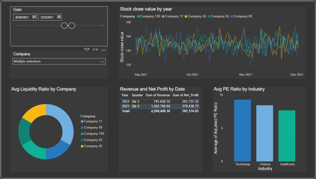
The aim of this project was to create some financial dashboards using Python, SQL and Power BI. Details on this project are below, but first, here are the results:

In order to achieve this I generated 3 years of financial data for 100 different non-existent companies using the following python script.
View code
num_companies = 100
start_date = '2020-01-01'
end_date = '2022-12-31'

dates = pd.date_range(start=start_date, end=end_date, freq='D')

# Company generation
company_names = [f'Company {i}' for i in range(1, num_companies + 1)]
industries = ['Technology', 'Healthcare', 'Finance', 'Energy']
company_data = pd.DataFrame({'Company': np.random.choice(company_names, num_companies),
                             'Industry': np.random.choice(industries, num_companies)})

# Random data generation within realistic ranges

size = len(dates) * num_companies

data = {
    'Date': np.tile(dates, num_companies),
    'Company': np.repeat(company_data['Company'], len(dates)),
    'Industry': np.repeat(company_data['Industry'], len(dates)),
    'Stock_Open': np.random.uniform(50, 200, size),  # Realistic stock price range
    'Stock_Close': np.random.uniform(50, 200, size),
    'PE_Ratio': np.random.uniform(5, 30, size),  # Realistic PE ratio range
    'PB_Ratio': np.random.uniform(0.5, 3, size),  # Realistic PB ratio range
    'Current_Assets': np.random.uniform(5000, 10000, size),  # Realistic current assets range
    'Current_Liabilities': np.random.uniform(3000, 8000, size),  # Realistic current liabilities range
    'Inventory': np.random.uniform(1000, 5000, size),  # Realistic inventory range
    'AR_Turnover': np.random.uniform(5, 20, size),  # Realistic accounts receivable turnover range
    'DSO': np.random.randint(20, 120, size),
    'Gross_Profit': np.random.uniform(1000, 5000, size),  # Realistic gross profit range
    'Net_Profit': np.random.uniform(500, 2000, size),  # Realistic net profit range
    'Total_Debt': np.random.uniform(2000, 8000, size),  # Realistic total debt range
    'Shareholders_Equity': np.random.uniform(2000, 10000, size),  # Realistic shareholders equity range
    'Operating_Cash_Flow': np.random.uniform(500, 2500, size),  # Realistic operating cash flow range
    'Cap_Expenditures': np.random.uniform(300, 1500, size),  # Realistic capital expenditures range
    'Revenue': np.random.uniform(1500, 8000, size),  # Realistic revenue range
    'EPS': np.random.uniform(1, 5, size)  # Realistic EPS range
}

# Create DataFrame
financial_data = pd.DataFrame(data)
As seen in the code, this would generate random data within specified ranges for the following financial metrics: Date, Company, Industry, Stock_Open, Stock_Close, PE_Ratio, PB_Ratio, Current_Assets, Current_Liabilities, Inventory, AR_Turnover, DSO, Gross_Profit, Net_Profit, Total_Debt, Shareholders_Equity, Operating_Cash_Flow, Cap_Expenditures, Revenue, EPS
This data was then migrated from the code output csv to SQL where I could conduct a few queries:
SELECT Industry, AVG(PE_Ratio) AS Avg_PE_Ratio, AVG(PB_Ratio) AS Avg_PB_Ratio
FROM financial_data
GROUP BY Industry;
The average PE Ratio (Price-to-Earnings Ratio) and average PB Ratio (Price-to-Book Ratio) are important financial indicators to assess the valuation and performance of companies within specific industries. The PE Ratio (which is calculated as Stock Price / Earnings Per Share) indicates the percieved value of a particular stock with a high PE ratio indiciating that investors have a high expectation of future growth.
The average PB Ratio (Price-to-Book value Ratio) compares the price of the stocks to the book value, which is assets – liabilities. Ratios higher or lower than 1 could indicate an over valuation or undervaluation respectively. This is more commonly used to value companies with tangible assets.
This simple query can can help to compare valuations, identify trends, support investment decisions and provide benchmarking statistics.
SELECT Company, SUM(Revenue) AS TotalRevenue
FROM financial_data
GROUP BY Company;
This similar query provides the total revenue generated for each company for all of the years of data included in the underlying tables.
SELECT Company, Stock_Open
FROM financial_data
WHERE Stock_Open > 180;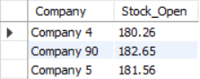
Filter queries like this are useful for extracting data from within specific parameters from large datasets like this.
SELECT Company, AVG(Stock_Open) AS AvgStockPrice
FROM financial_data
WHERE Date BETWEEN '2020-01-01' AND '2021-01-01'
GROUP BY Company;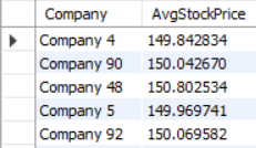
Here I have calculated the average stock price for each company over the specified period.
To make the data more visually pleasing and to provide a way to dynamically explore the data I linked this SQL database to Power BI, where I generated the dashboards at the top of this page as an example of some of the ways in which financial data between different companies and industries can be easily viewed and compared.
